Reference website1:
MS Excel Tutorial - Formulas

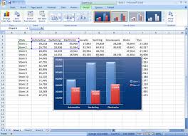
MS excel addition with images:


 Functions A function, such as PI(), starts with an equal sign (=), and you can enter arguments for the function within its parentheses. Each function has a specific argument syntax.
 Cell references You can refer to data in worksheet cells by including cell references in the formula. For example, the cell reference A2 returns the value of that cell or uses that value in the calculation.
 Constants You can also enter constants, such as numbers (such as 2) or text values, directly into a formula.
 Operators Operators are the symbols that are used to specify the type of calculation that you want the formula to perform. For example, the ^ (caret) operator raises a number to a power, and the * (asterisk) operator multiplies numbers.
 The first cell reference is B3, the color is blue, and the cell range has a blue border with square corners. The second cell reference is C3, the color is green, and the cell range has a green border with square corners.
 The AVERAGE and SUM functions are nested within the IF function.


MS Excel Tutorial - Formulas
Tags:excel formulas,ms excel formulas,ms excel latest formulae,excel latest formulae,ms excel fundamentals,
ms excel manual free download,ms excel e books torrent download, ms excel with neat images,learn ms excel yourself, learn ms excel, ms excel sum formula,easy step to learn ms office with images,

Reference website2:
Excel Formulas - Microsoft Excel Formulas - Excel Formulas Tutorial

Official Microsoft website link:
Create a formula - Excel - Microsoft Office

Excel 2010- For Dummies Quick Reference.pdf Torrent Download
.
ms excel manual free download,ms excel e books torrent download, ms excel with neat images,learn ms excel yourself, learn ms excel, ms excel sum formula,easy step to learn ms office with images,
Reference website2:
Excel Formulas - Microsoft Excel Formulas - Excel Formulas Tutorial
Official Microsoft website link:
Create a formula - Excel - Microsoft Office
Excel 2010- For Dummies Quick Reference.pdf Torrent Download
.
Excel Formulas Overview
Related Tutorial: Excel 2010 and 2007 Formulas Tutorials.
This tutorial covers in detail how to create and use formulas, including a step by step example of a basic Excel formula. It is intended for those with little or no experience in working with spreadsheet programs such as Excel.
Click on the links below to read specific information.
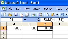
MS excel subtraction with images:
MS excel multiplicatoin with images:
MS excel Division with images:
- Writing the Formula - How to enter a formula
- Cell References in Formulas - Make it easy to change your spreadsheet
- Updating Excel Formulas - Automatic updating
- Mathematical Operators in Formulas- Adding to formulas
- Excel Formulas Tutorial Step 1- Entering the Data
- Excel Formulas Tutorial Step 2 - Add the Equal (=) Sign
- Excel Formulas Tutorial Step 3 - Add Cell References Using Pointing
Formulas are equations that perform calculations on values in your worksheet. A formula always starts with an equal sign (=).
You can create a simple formula by using constants and calculation operators. Simple formulas can include values you enter, cell references, or names you have defined. For example, =A1+A2 or =5+2 are simple formulas that add the values in cells A1 and A2 or the values that you specify.
You can also create a formula by using a function. For example, the formulas=SUM(A1:A2) and SUM(A1,A2) both use the SUM function to add the values in cells A1 and A2. In addition to formulas that use a single function, you can create formulas with nested functions or arrays that calculate single or multiple results.
NOTE This article provides procedures for creating different formulas. For examples of formulas, see Examples of commonly used formulas. For more information about deleting or removing formulas, see Delete or remove a formula.
What do you want to do?
- Learn about the parts of a formula
- Create a simple formula by using constants and calculation operators
- Create a formula by using cell references and names
- Create a formula by using a function
- Create a formula by using nested functions
- Create an array formula that calculates a single result
- Create an array formula that calculates multiple results
- Learn tips and tricks about creating formulas
- Avoid common errors when creating formulas
Learn about the parts of a formula
Depending on the type of formula that you create, a formula can contain any or all of the following parts:
Functions A function, such as PI(), starts with an equal sign (=), and you can enter arguments for the function within its parentheses. Each function has a specific argument syntax. Cell references You can refer to data in worksheet cells by including cell references in the formula. For example, the cell reference A2 returns the value of that cell or uses that value in the calculation. Constants You can also enter constants, such as numbers (such as 2) or text values, directly into a formula. Operators Operators are the symbols that are used to specify the type of calculation that you want the formula to perform. For example, the ^ (caret) operator raises a number to a power, and the * (asterisk) operator multiplies numbers.
Create a simple formula by using constants and calculation operators
- Click the cell in which you want to enter the formula.
- Type = (equal sign).
- To enter the formula, do one of the following:
- Type the constants and operators that you want to use in the calculation.
| EXAMPLE FORMULA | WHAT IT DOES |
|---|---|
| =5+2 | Adds 5 and 2 |
| =5-2 | Subtracts 2 from 5 |
| =5/2 | Divides 5 by 2 |
| =5*2 | Multiplies 5 times 2 |
| =5^2 | Raises 5 to the 2nd power |
- Click the cell that contains the value that you want to use in the formula, type the operator that you want to use, and then click another cell that contains a value.
| EXAMPLE FORMULA | WHAT IT DOES |
|---|---|
| =A1+A2 | Adds the values in cells A1 and A2 |
| =A1-A2 | Subtracts the value in cell A2 from the value in A1 |
| =A1/A2 | Divides the value in cell A1 by the value in A2 |
| =A1*A2 | Multiplies the value in cell A1 times the value in A2 |
| =A1^A2 | Raises the value in cell A1 to the exponential value specified in A2 |
- Press ENTER.
Tips
- You can enter as many constants and operators as you need to achieve the calculation result that you want.
- Excel follows the standard order of mathematical operations. For example, the formula =5+2*3, multiplies two numbers and then adds a number to the result – the multiplication operation (2*3) is performed first, and then 5 is added to its result.
Create a formula by using cell references and names
The example formulas at the end of this section contain relative references to and names of other cells. The cell that contains the formula is known as a dependent cell when its value depends on the values in other cells. For example, cell B2 is a dependent cell if it contains the formula =C2.
- Click the cell in which you want to enter the formula.
- In the formula bar
 , type = (equal sign).
 - Do one of the following:
- To create a reference, select a cell, a range of cells, a location in another worksheet, or a location in another workbook. This behavior is called semi-selection. You can drag the border of the cell selection to move the selection, or drag the corner of the border to expand the selection.
The first cell reference is B3, the color is blue, and the cell range has a blue border with square corners. The second cell reference is C3, the color is green, and the cell range has a green border with square corners. NOTE If there is no square corner on a color-coded border, the reference is to a named range.
- To enter a reference to a named range, press F3, select the name in the Paste name box, and click OK.
| EXAMPLE FORMULA | WHAT IT DOES |
|---|---|
| =C2 | Uses the value in the cell C2 |
| =Sheet2!B2 | Uses the value in cell B2 on Sheet2 |
| =Asset-Liability | Subtracts the value in a cell named Liability from the value in a cell named Asset |
- Press ENTER.
For more information, see Create or change a cell reference or Define and use names in formulas.
Create a formula by using a function
- Click the cell in which you want to enter the formula.
- To start the formula with the function, click Insert Function
 on the formula bar .
 - Select the function that you want to use.
You can enter a question that describes what you want to do in the Search for a function box (for example, "add numbers" returns the SUM function), or browse from the categories in the Or Select a category box.
TIP For a list of available functions, see List of worksheet functions (alphabetical)or List of worksheet functions (by category).
- Enter the arguments.
TIP To enter cell references as an argument, click Collapse Dialog  (which temporarily hides the dialog box), select the cells on the worksheet, and then press Expand Dialog
  .
.
(which temporarily hides the dialog box), select the cells on the worksheet, and then press Expand Dialog .| EXAMPLE FORMULA | WHAT IT DOES |
|---|---|
| =SUM(A:A) | Adds all numbers in column A |
| =AVERAGE(A1:B4) | Averages all numbers in the range |
- After you complete the formula, press ENTER.
TIP To summarize values quickly, you can also use AutoSum. On the Home tab, in the Editing group, click AutoSum, and then click the function that you want.
Create a formula by using nested functions
Nested functions use a function as one of the arguments of another function. You can nest up to 64 levels of functions. The following formula sums a set of numbers (G2:G5) only if the average of another set of numbers (F2:F5) is greater than 50. Otherwise, it returns 0.
The AVERAGE and SUM functions are nested within the IF function.- Click the cell in which you want to enter the formula.
- To start the formula with the function, click Function Wizard on the formula bar .
- Select the function that you want to use.
You can enter a question that describes what you want to do in the Search for a function box (for example, "add numbers" returns the SUM function), or browse from the categories in the Or Select a category box.
TIP For a list of available functions, see List of worksheet functions (alphabetical)or List of worksheet functions (by category).
- To enter the arguments, do one or more of the following:
- To enter cell references as an argument, click Collapse Dialog next to the argument you want (which temporarily hides the dialog box), select the cells on the worksheet, and then press Expand Dialog .
- To enter another function as an argument, enter the function in the argument box that you want. For example, you can add SUM(G2:G5) in the Value_if_true edit box of the IF function.
- The parts of the formula displayed in the Function Arguments dialog box reflect the function that you selected in the previous step. For example, if you clicked IF, the Function arguments dialog box displays the arguments for the IF function.
Create an array formula that calculates a single result
You can use an array formula to perform several calculations to generate a single result. This type of array formula can simplify a worksheet model by replacing several different formulas with a single array formula.
- Click the cell in which you want to enter the array formula.
- Enter the formula that you want to use.
TIP Array formulas use standard formula syntax. They all begin with an equal sign, and you can use any of the built-in Excel functions in your array formulas.
For example, the following formula calculates the total value of an array of stock prices and shares, without using a row of cells to calculate and display the total values for each stock.
Array formula that produces a single result
When you enter the formula {=SUM(B2:C2*B3:C3)} as an array formula, Excel multiples the number of shares by the price for each stock (500*10 and 300*15), and then adds the results of those calculations together to get a total value of 9500.
- Press CTRL+SHIFT+ENTER.
Excel automatically inserts the formula between { } (a pair of opening and closing braces).
NOTE Manually typing braces around a formula will not convert it into an array formula — you must press CTRL+SHIFT+ENTER to create an array formula.
IMPORTANT Any time you edit the array formula, the braces ({ }) disappear from the array formula, and you must press CTRL+SHIFT+ENTER again to incorporate the changes into an array formula and to add the braces.
Create an array formula that calculates multiple results
Some worksheet functions return arrays of values, or require an array of values as an argument. To calculate multiple results by using an array formula, you must enter the array into a range of cells that has the same number of rows and columns as the array arguments have.
- Select the range of cells in which you want to enter the array formula.
- Enter the formula that you want to use.
TIP Array formulas use standard formula syntax. They all begin with an equal sign, and you can use any of the built-in Excel functions in your array formulas.
For example, given a series of three sales figures (column B) for a series of three months (column A), the TREND function determines the straight-line values for the sales figures. To display all of the results of the formula, it is entered into three cells in column C (C1:C3).
Array formula that produces multiple results
When you enter the formula =TREND(B1:B3,A1:A3) as an array formula, it produces three separate results (22196, 17079, and 11962), based on the three sales figures and the three months.
- Press CTRL+SHIFT+ENTER.
Excel automatically inserts the formula between { } (a pair of opening and closing braces).
NOTE Manually typing braces around a formula will not convert it into an array formula — you must press CTRL+SHIFT+ENTER to create an array formula.
IMPORTANT Any time you edit the array formula, the braces ({ }) disappear from the array formula, and you must press CTRL+SHIFT+ENTER again to incorporate the changes into an array formula and to add the braces.
Learn tips and tricks about creating formulas
When you work with formulas, it’s good to know how you can easily change the type of reference the formula is using, copy formulas to other cells in the worksheet, avoid formula errors by using Formula Autocomplete, and take advantage of Function Screen tips that are provided for each function to learn more about the formula arguments.
SWITCH BETWEEN RELATIVE, ABSOLUTE, AND MIXED REFERENCES
To switch between relative, absolute, and mixed references:
- Select the cell that contains the formula.
- In the formula bar , select the reference that you want to change.
- Press F4 to switch between the reference types.
For more information about switching between reference types, see Switch between relative, absolute, and mixed references.
QUICKLY COPY FORMULAS TO OTHER CELLS
You can quickly enter the same formula into a range of cells. Select the range that you want to calculate, type the formula, and then press CTRL+ENTER. For example, if you type =SUM(A1:B1) in range C1:C5, and then press CTRL+ENTER, Excel enters the formula in each cell of the range, using A1 as a relative reference.
You can also use the Fill command to copy formulas into adjacent cells. For more information, see Fill data automatically in worksheet cells.
USE FORMULA AUTOCOMPLETE
To make it easier to create and edit formulas and minimize typing and syntax errors, use Formula Autocomplete. After you type an = (equal sign) and beginning letters, Excel displays a dynamic list of valid functions and names below the cell. After you insert the function or name into the formula by pressing TAB or double-clicking the item in the list, Excel displays any appropriate arguments. As you fill out the formula, typing a comma can also display additional arguments. You can insert additional functions or names into your formula and, as you type their beginning letters, Excel again displays a dynamic list from which you can choose.
Formula Autocomplete is on by default. To turn it on or off, see Use Formula AutoComplete.
USE FUNCTION SCREENTIPS
If you are not familiar with the arguments of a function, you can use the function ScreenTip that appears after you type the function name and an opening parenthesis. Click the function name to view the Help topic on the function, or click an argument name to select the corresponding argument in your formula.
Avoid common errors when creating formulas
The following table summarizes some of the most common mistakes you can make when entering a formula and how to avoid formula errors:
| MAKE SURE THAT YOU… | MORE INFORMATION |
|---|---|
| Match all open and close parentheses in the formula | All parentheses are part of a matching pair in formulas. When you create a formula, Excel displays parentheses in color as they are entered. |
| Use a colon to indicate a range you enter in the formula | Colons (:) are used to separate the reference to the first and last cell in the range. For example, A1:A5. |
| Enter all required arguments | Functions can have required and optional arguments (indicated by square brackets in the syntax). All required arguments should be entered. Also, make sure that you have not entered too many arguments. |
| Do not nest more than 64 functions in a formula | Nesting functions within a formula is limited to 64 levels. |
| Enclose workbook or worksheet names in single quotation marks | When referring to values or cells on other worksheets or workbooks that have non-alphabetical characters in their names, the names must be enclosed in single quotation marks ( ' ). |
| Include the path to external workbooks | External references must contain a workbook name and the path to the workbook. |
| Enter numbers without formatting | Numbers you enter in a formula should not be formatted with decimal separators or dollar signs ($) because commas are already used as argument separators in formulas, and dollar signs are used to mark absolute references. For example, instead of entering $1,000, enter1000 in the formula. |
excel formulas
A forumla is nothing more than an equation that you write up. In Excel a typical formula might contain cells, constants, and even functions. Here is an example Excel formula that we have labeled for your understanding.
=B3 * 5 / SUM(B4:B7)
- cell(s): B3 and the range of cells from B4:B7
- constant(s): 5
- function(s): SUM()
excel formulas: creating your first formula
This first formula will be as simple as they come and will teach you the basic form of an Excel formula. Create a new spreadsheet and then follow these steps:
- Select cell A1
- Type the following basic arithmetic formula into cell A1: =1+1

- Press Enter and notice how cell A1 changes from your formula to the result!
This may seem simple, but there are a some very important things you should get out of this example. When you start off a cell entry with the equal sign "=" you are telling Excel that you want it to evaluate the following formula.
In our case we had a simple "1+1" we wanted Excel to solve for us. You can do this for addition, subtraction, multiplication, division and any other operation you can think of.
Remember, if you do not start your entry with the equal sign, then Excel will not evaluate the cell!
using cells to create dynamic formulas
The most powerful aspect of Excel is not the simple calculator abilities we describes in our first formula example, but rather the ability to take values from cells to be used in your formulas.
Let's set up a basic sales spreadsheet to help explain this topic.
- In cells A1-D4 enter the following information:
Notice: that cell D2 and D3 are blank, but should contain the amount of money from selling 150 candy items and 3 vegetables. By referencing the Quantity and Price cells we will be able to do this! Let's begin with Candy. - Note:It is very important to follow these steps exactly without interruptions! Select cell D2, candy's "revenue", and type the equal sign "=" to begin your formula.
- Left-click on cell B2, Candy's Quantity and notice your formula is now "=B2"

- We want to multiply Quanity(B2) by Price(B3) so enter an asterisk (*)
- Now left-click on Candy's Price (C2)to complete your formula!
- If your formula looks like ours then press Enter, otherwise you can manually enter the formula "=B2*C2". However, we really think it is easier and preferred to click on cells to reference them, instead of entering that information manually.
- After you pressed Enter your Candy Revenue cell should be functioning properly and contain the value 75.

- Using your newly gained knowledge please complete Vegetable's Revenue by repeating steps 2-7 for Vegetable
- Your spreadsheet should now look like this:
- Cheatsheet: If you are having trouble creating the formula for Vegetable's Revenue it is "=B3*C3"
advanced excel formulas: using formulas in formulas
Now that we have created separate revenues for both Candy and Vegetable it would be nice to somehow combine these two values to get the Total Revenue. Although both Vegetable Revenue and Candy Revenue contain formulas, we can still use these cells as we have been doing and add them together to get our total.
- Select cell D5 (directly below "Total")
- Type the equal sign "="
- Left-click cell D2
- Type the plus sign "+"
- Left-click cell D3. Cell D5 should now contain this formula "=D2+D3":
- Press Enter to complete your Total Revenue!